Land use change is a complex process affected by countless factors. It is considered to be one of the most impactful drivers of climate change. Land use change can be defined as any kind of human activity that manipulates land. Ecosystems are proven to be higly susceptible to human intervention. Ecosystems are crucial in keeping the balance of the earth's surface and underground stability. So what can be done to make land use change less impactful in terms of impact on ecosystems? Understanding land use change dynamics and patterns might help countries to implement higher levels of infrastructure organization. So how can land use change dynamics can be understood? Let's scroll down and take a look at how it changes in time.

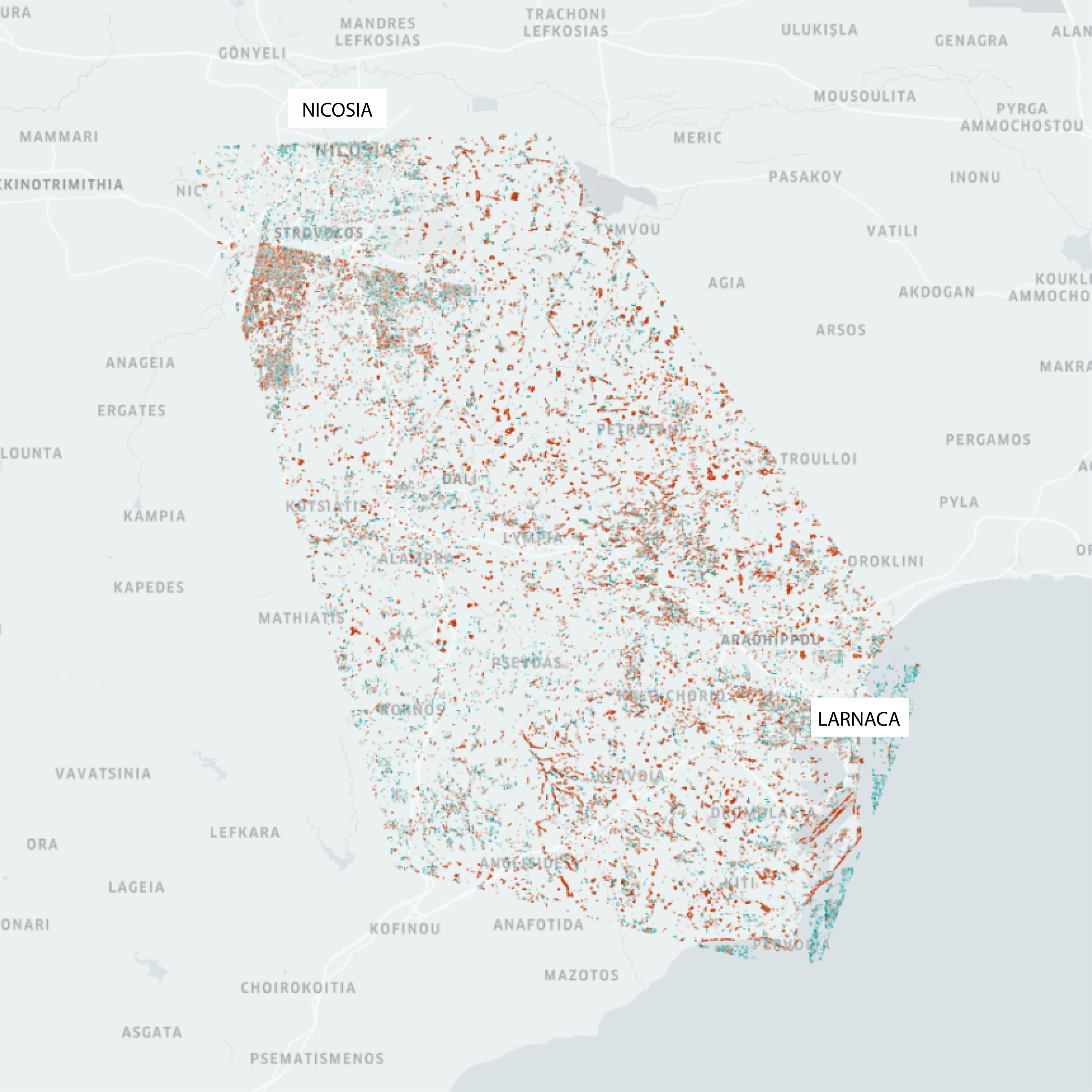
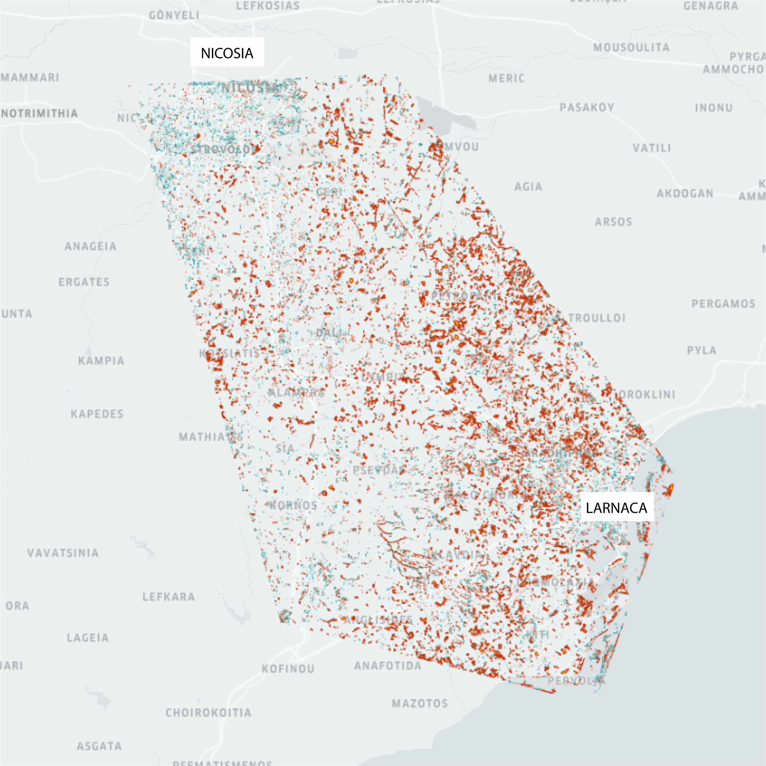
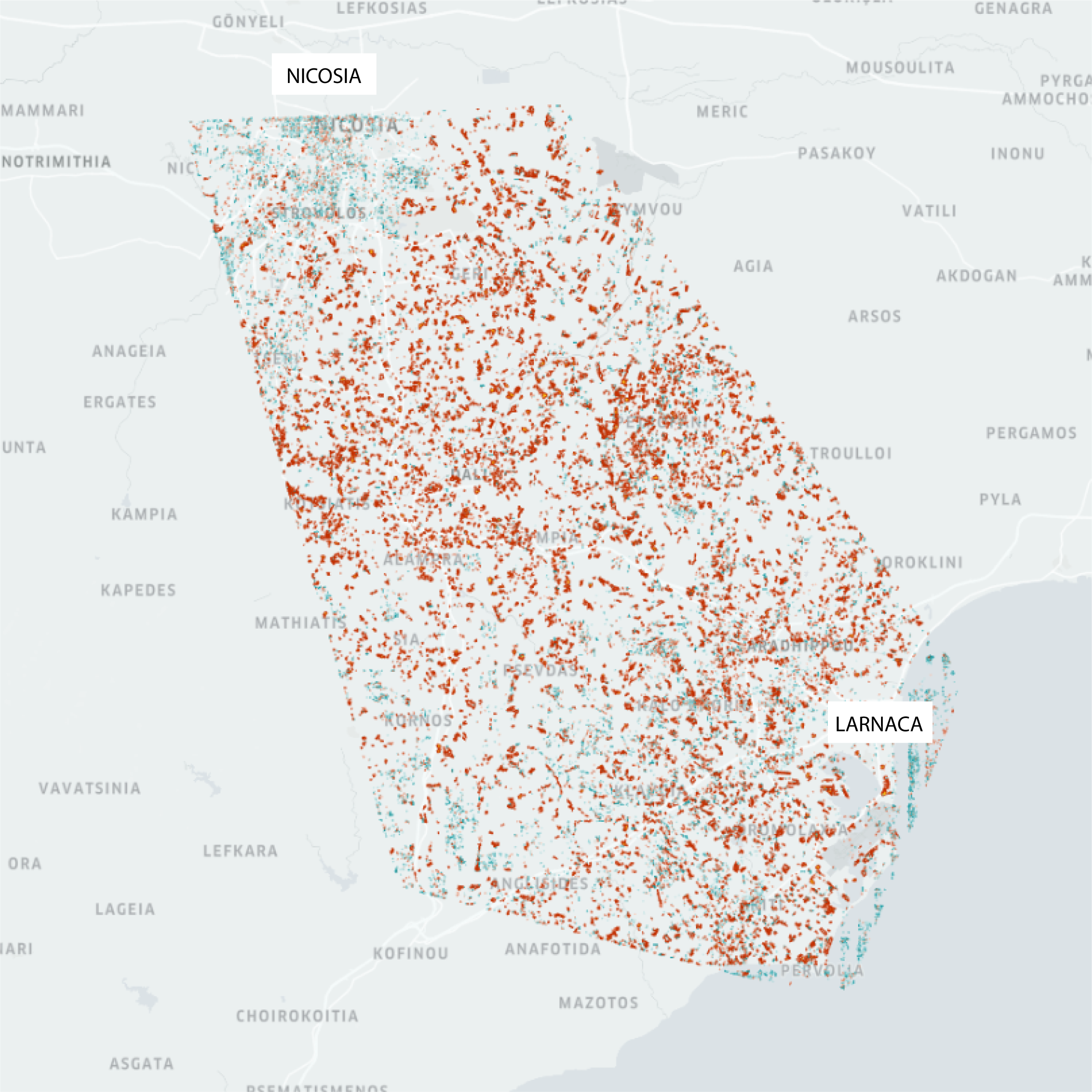
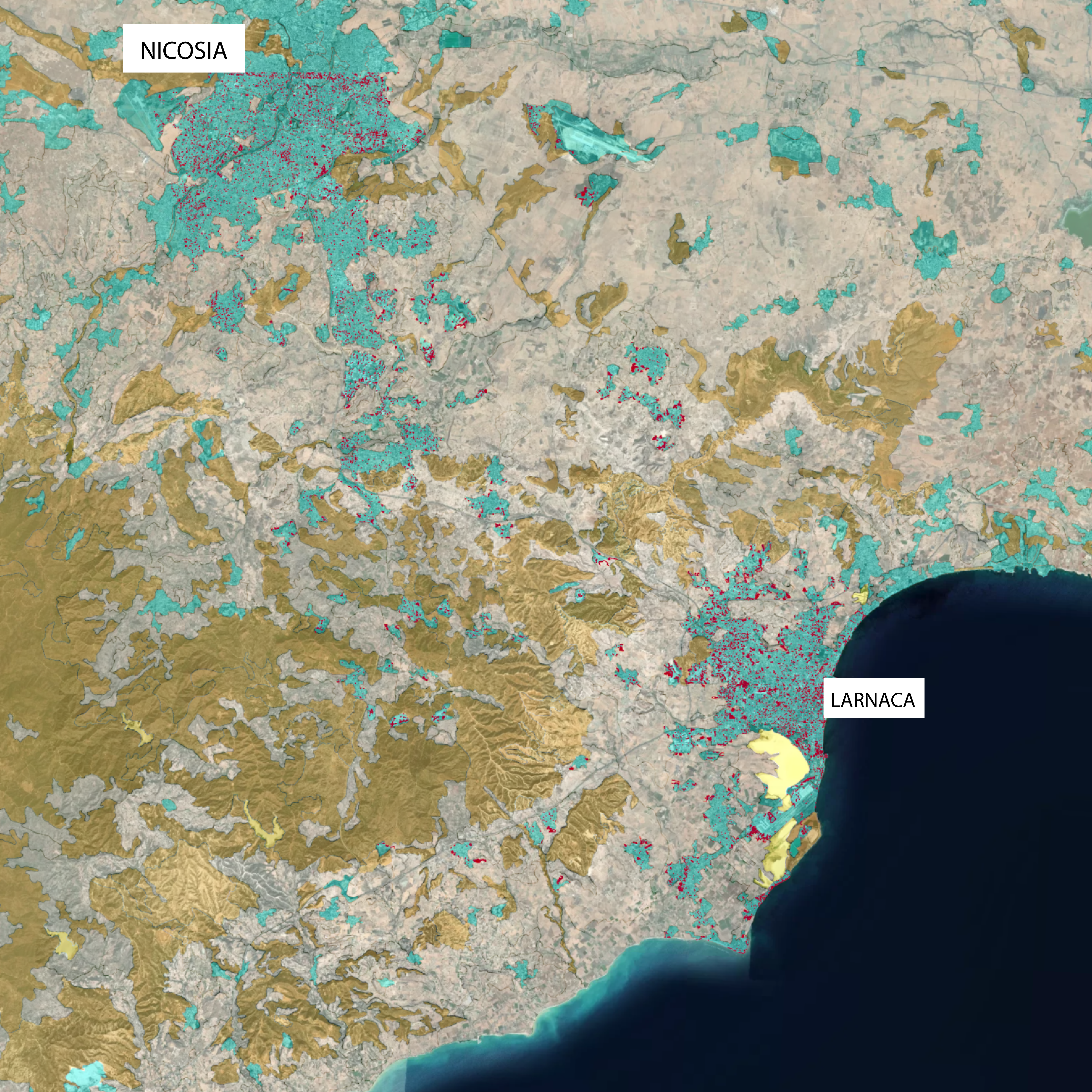
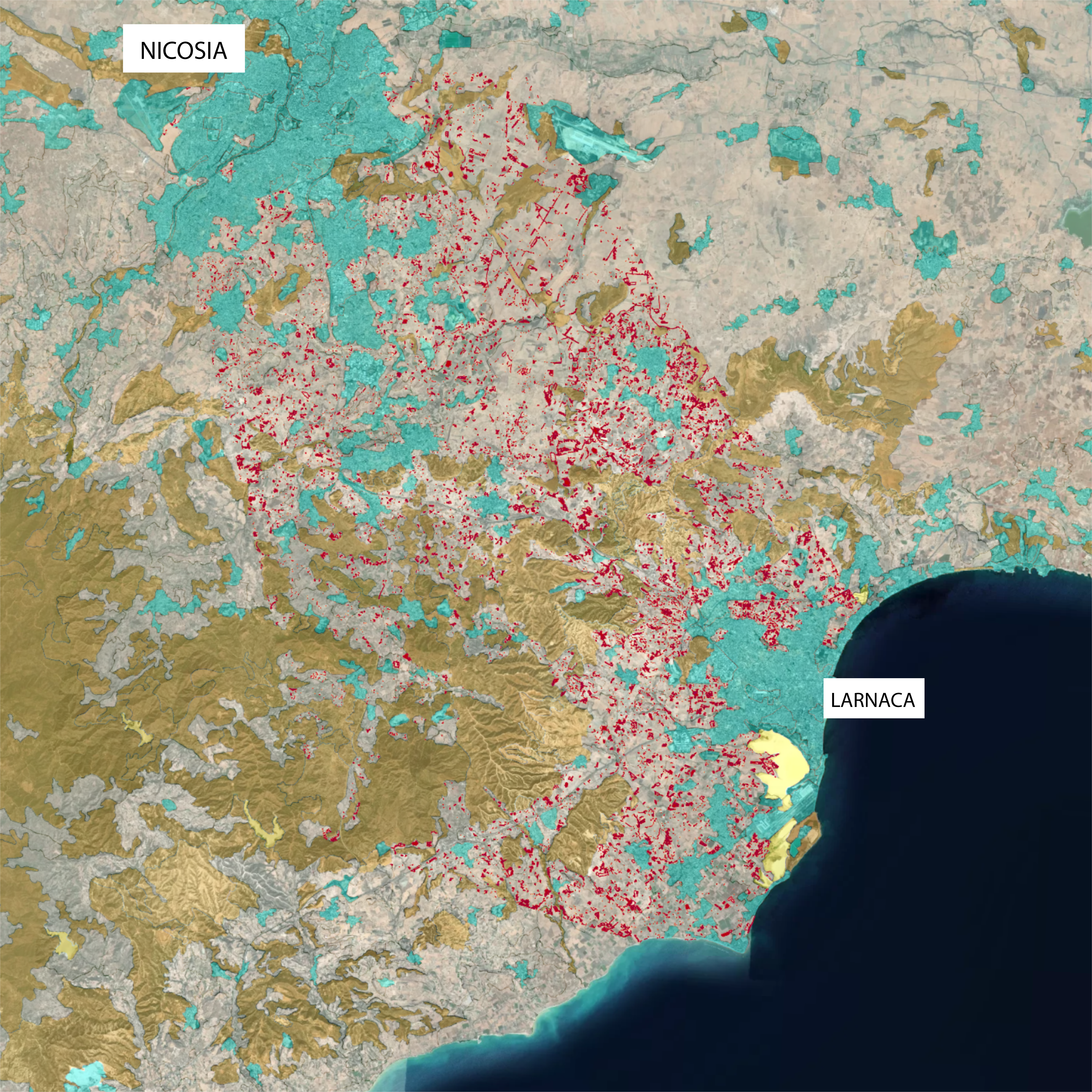
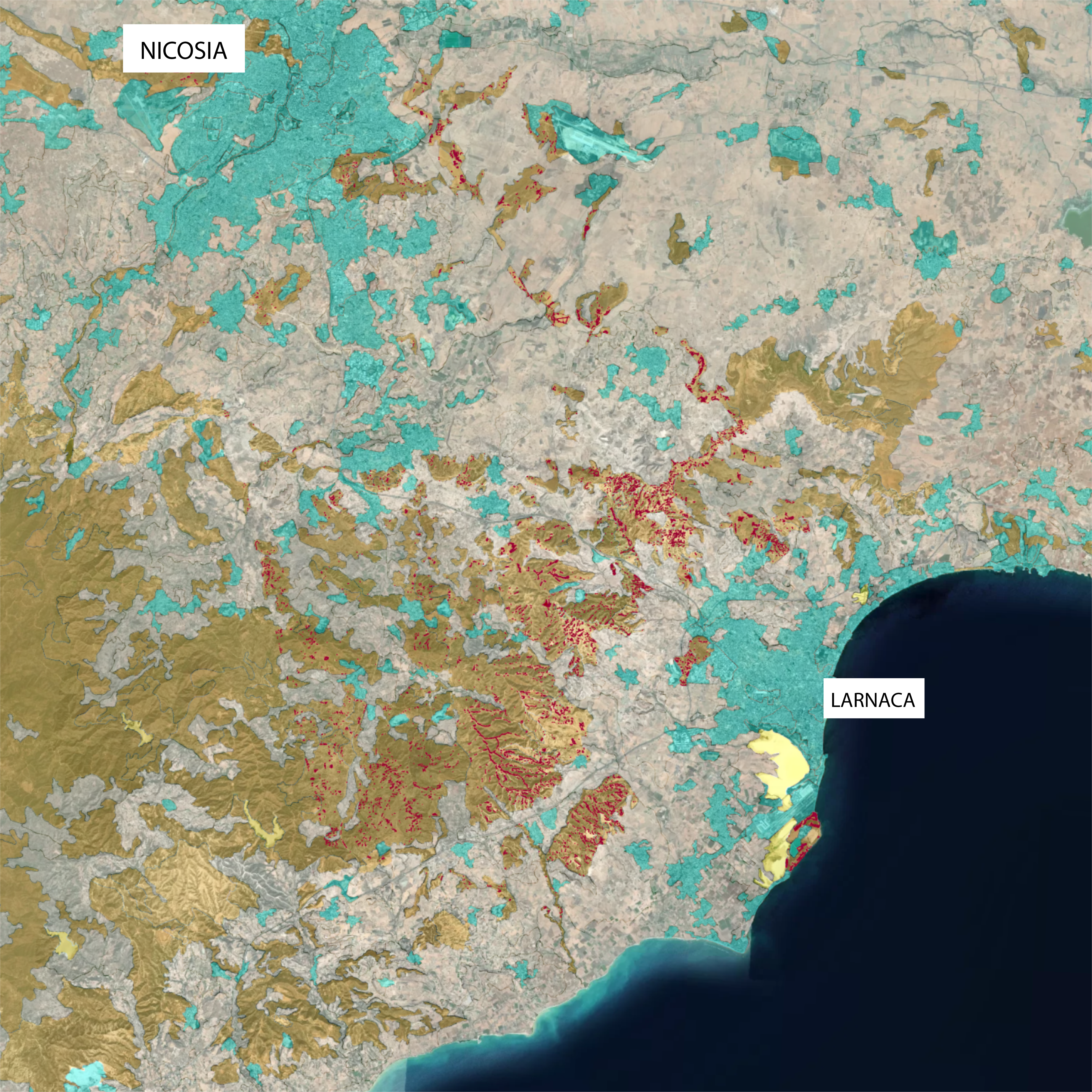
The following visualization shows the plot of raw detected land use change in three different moments in time. Each visualization shows a change detected in a timeframe of two weeks each, and the respective dates are 15th of February (first), 5th of March (second), and 30th of March (third). Two key points can be stated: the change in cities and the change in rural areas do not behave in the same way. Cities present a way granular and smaller sized type of land use change. Second, there is a big increase in rural activity in the transition from February to March, or from winter to spring. To emphasise the transition, the colors are determined by the size of detected change (blue - smaller, red - bigger).

February 15th

March 5th

March 30th

link to the interactive version

The following visualization (interactive) brings the analysis to the next step. Through the use of geoprocessing and clustering features, it becomes more evident how the change distributes across the studied region in time. The visualizations subdivide the data in a fishernet grid, and each cell of the grid is represented by one of the three colors: blue, grey, and red. These colors are determined by the z-score of the hotspot analysis. Hotspot analysis calculates the amount of data points in each cell and returns a corresponding z-score. A low z-score (negative) is represented the blue color and means that a relatively small amount of change has been detected in those area (compared to all the other areas analyzed). A medium z-score (close to zero) is represented by the grey color, and means that the amount of change in the area is average or statistically insignificant. Finally, a high z-score (positive) is represented by the red color and means that a high amount of land use change has been detected. The areas just described can be also named as cold spots, not significant, and hot spots. The bottom graphs represent the plot of the sums of different statistical regions, which put further emphasis on the seasonal transition.

In the next visualization (interactive), the hotspot analysis is performed on the totality of the data, or the entire 6 week timeframe. The aim of this is to further study the concentration of land use change over a longer period of time. As it can be seen, urban areas present a higher amount of single/separate land use changes.

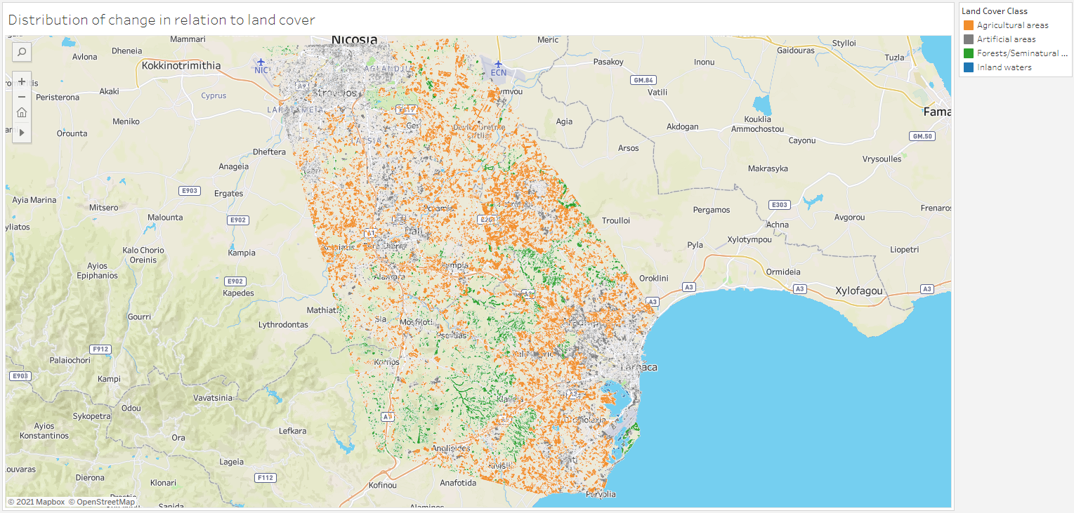
The next visualization plots the totality of the dataset (entire 6 week timeframe) in correlation to the CORINE Land cover dataset. The aim of the visualization is to further study the distribution of land use change in correlation to previously released map of european land cover, to understand how land use change distributes, for instance, in urban or in agricultural areas.

March 30th

link to the interactive version

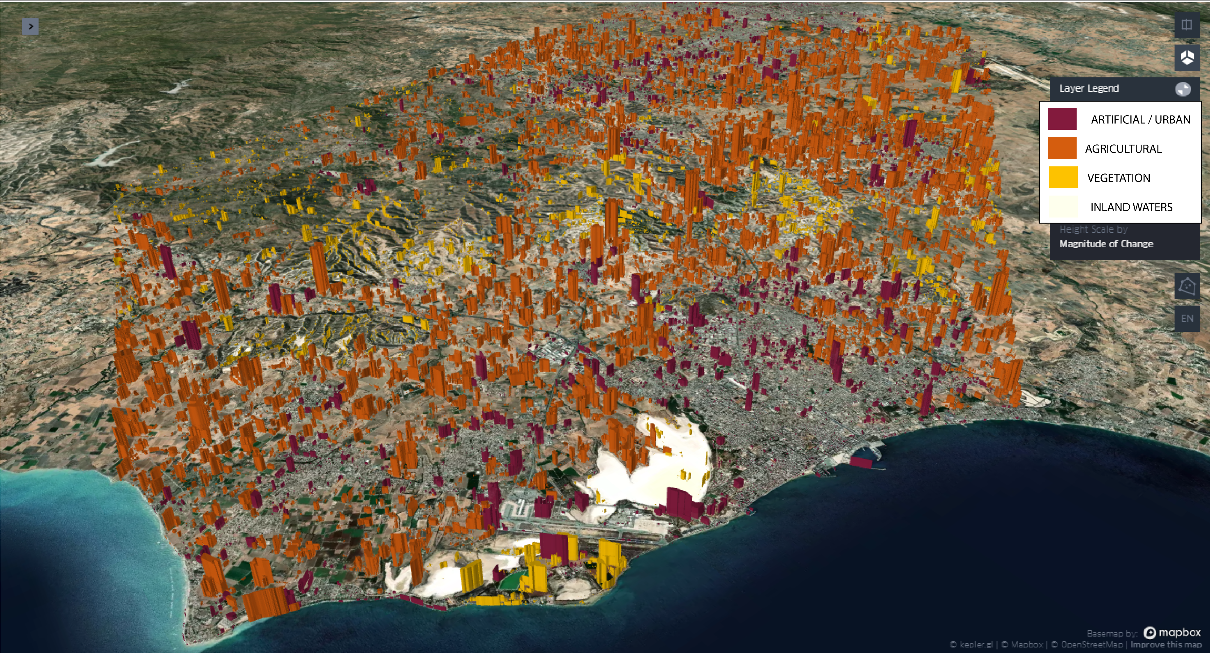
The following visualization extends the previous one, and shows the plot of the detected land use change above the plot of the CORINE dataset. The red marks represent the detected land use change, while the 4 different colors coloring the surface of the map represent the four different categories of land cover: artificial, agricultura, forests, and inland waters.

The following visualization plots polygons over the detected land use change, and the height of each polygon is determined by the surface area covered by the specific change. The aim of this graph is to study the distribution of land from the magnitude perspective. The plot shows that the detected land use change of greated magnitues (higher amount of squared kilometers) tend to concentrate in agricultural areas. The four different colors are, again, represented by the differend land cover types.

link to the interactive version

The following dashboard depicts the two different analyses focused on the two distinct urban areas, Nicosia and Larnaka. The first analysis (top) shows the hotspot analysis performed on the size of each detected change. The second analysis (bottom) represent the hotspot analysis performed on the each single position of detected land use change (same as the graphs above). The colors are, once again, determined by the z-score, and the aim of the graph is to confirm that the change inside cities is more granular and more occurent, while the change outside of the cities is greated in area coverage.
The z-score, as mentioned above, is a way to see where the most occurences of a specific variable takes place. In this case, in the above graphs the z-score is determined by the size of detected change, and thus shows where the largest change is most likely to occur. On the other size, the bottom graphs' z-score is determined by the position of each single detected change and, thus, show where most of the single land use changes are most likely to occur. The interactive maps allow to visualize the legend, switch basemap, and switch layers (bottom, switch between hotspot and density analysis).

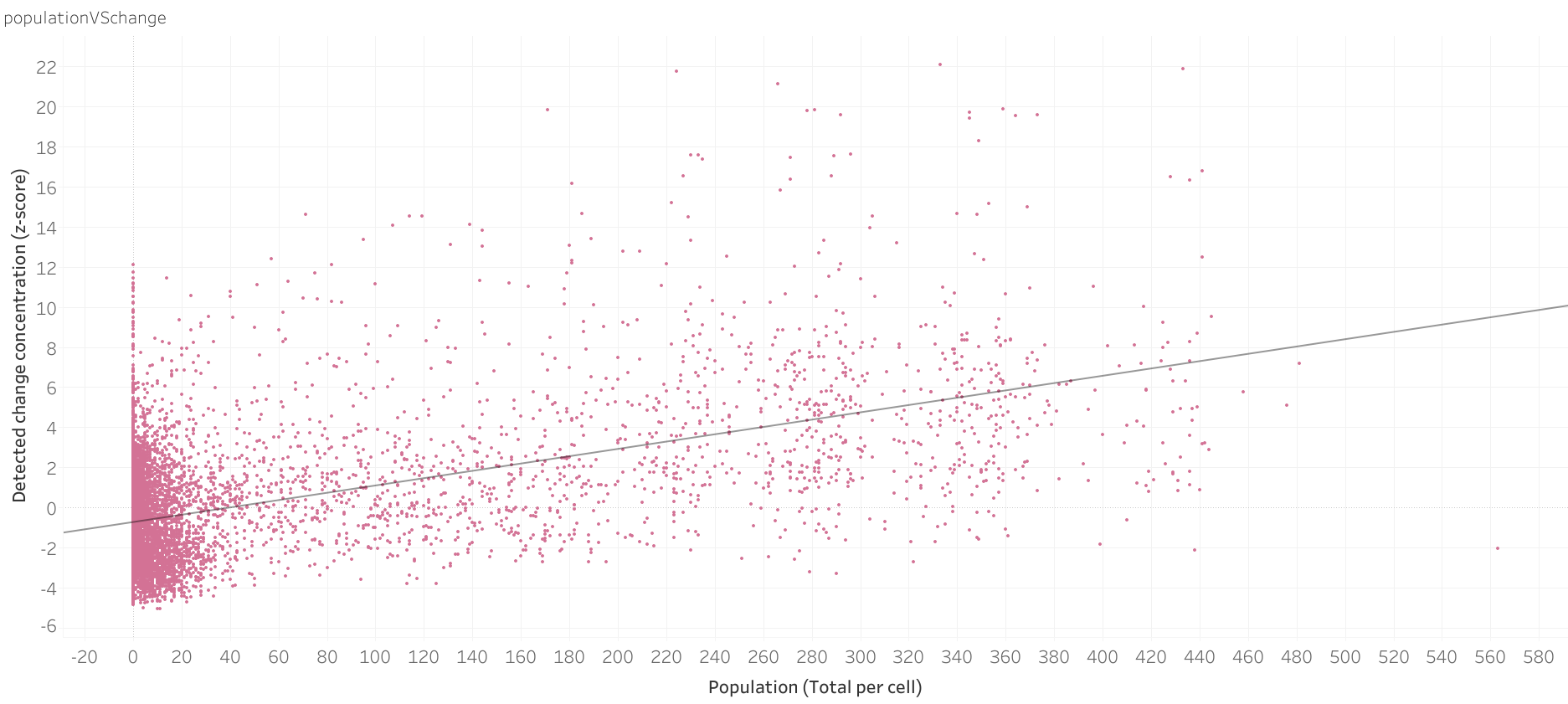
The following graphs focus on studying land use change in correlation to demographic factors. All the demographic datasets are provided by ESRI. The following visualization shows the correlation between population and the distribution of change. the X axis represent the population number in a specic cell, while the Y axis represents the z-score of that specific cell. For example, in previous graphs we've seen the plots of the z-score on the map, where areas colored in red represented a higher probability of multiple land use changes to occur. This areas, in the current graph, are now visualized in a scatter plot, and the data points of such red areas will reside in a higher position along the Y axis, while the population number in the range of that red area will determine the X value.
The population shows a clear uptrend towards hotspots, which indicates that most of the population tends to concentrate in urban areas (highest z-scores were shown to be located in urban areas in the previous graphs).

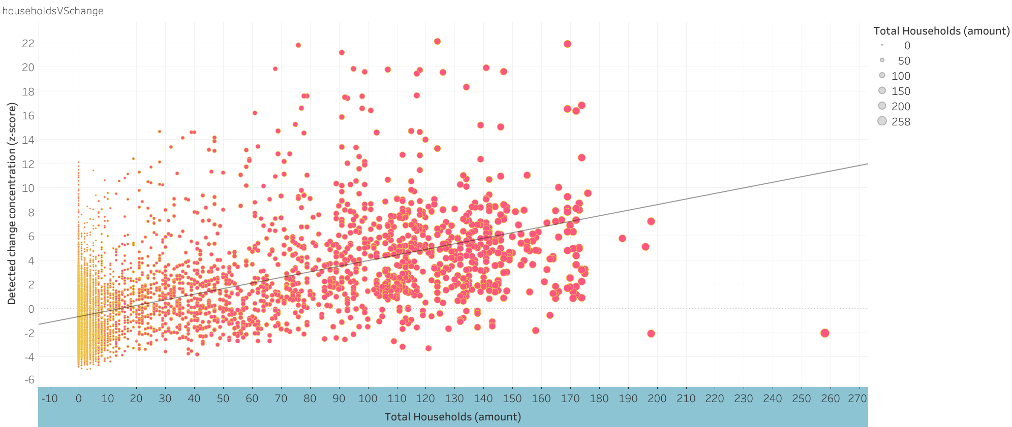
The following graph represents the correlation between the amount of households and the distribution of land use change. In a similar way, here the X axis is represented by the amount of households in a specific cell, while the Y axis is represented by the z-score of that specific cell. Once again, an uptrend can be observer, which means that higher amounts of households tend to be located around urban areas.

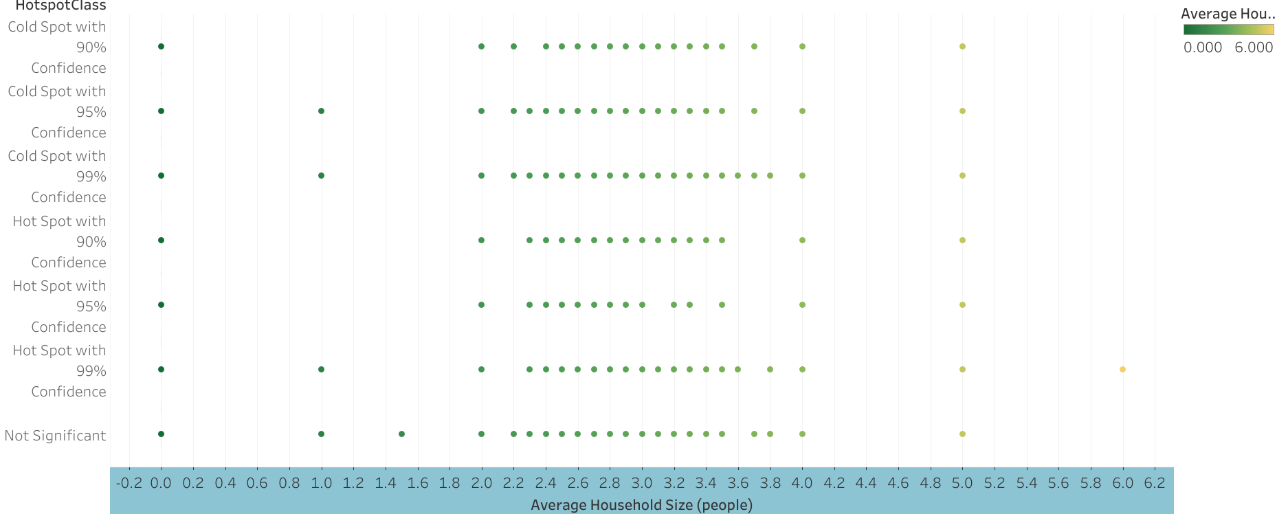
The next graph compares the z-scores (Y axis) with the average household sizes (X axis). A cold spot is represented by a low z-score, while a hot spot is represented by a high z-score. This graph shows that the average household size is, more or less, equally distributed across the whole analyzed area and, thus, doesn't seem to affect land use change in any way.

The following three visualizations are exploratory and give the possibility to autonomously swtich between different demographic factors. The first one compares the z-scores (Y axis) with a chosen demographic factor in a scatter plot. The 3 distinct areas are filtered for Each plot and are the cold spots, hotspots, and not significant spots. As mentioned before, a hotspot is represented by a high z-score, and indicates a high probability of land change happening, while the coldspot is represented by a low (below zero) z-score and indicates a low probability of land change happening.

The next graph compares the ditribution of two different demographic factors in relation to the z-score in a linear plot.

The last graph compares two different demographic factors (Y axis) in correlation with the size of detected change (CLUSTER_POINT_COUNT, X axis). Furthermore, the band plot is divided in the four different land cover categories. The aim is to further observe the connection betweeen land use change, demographic factors, and land cover.
The CLUSTER_POINT_COUNT, as previously mentioned, represents the size of the detected change (alternativly to squared kilometers for technical reasons).